4.1 Comparability of the Sentiment Lexicons

In the beginning we wanted to assess if the different lexica sentiment scores for tweets were actually comparable. For that purpose we computed the correlation between tweet sentiment scores provided by each pair of sentiment lexica to assess whether the ranking of the tweets according to one sentiment lexicon agrees with the ranking of the tweets according to another sentiment lexicon.

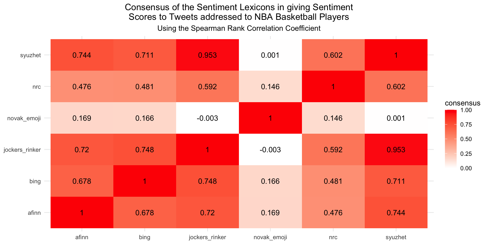
Generally we can see that except of the Emoji Sentiment Lexicon by Novak all other sentiment lexicons seem to correlate rather well. Apparently the computed tweet sentiments from the Emoji Lexicon differ strongly from the sentiments of the other lexica which is reasonable since the Emoji Lexicon is only computed on the emojis contained in the tweet while the other lexica use the textual information of the tweet. The Jockers Rinker and Syuzhet lexicons are most similar with a correlation coefficient around 0.95. This intuitively also makes sense since Jockers-Rinker is a combined version of Syuzhet and Bing as mentioned before.

4.2 Computing Sentiment Aggregates

Since the sentiment scores were computed on a per-tweet basis we first had to aggregate the sentiment scores accordingly in order to capture the overall social media vibe, players were receiving. For that purpose we considered the sentiment scores of all tweets a player received in a 24 hour window before a game and aggregated them as follows:

• The average of the sentiment scores (mean)
• The average of the sentiment scores weighted by the retweet count of the associated tweet (weighted mean)
• The proportion of tweets with a negative associated sentiment score (< 0)

4.3 Distribution of the Sentiment Aggregates and BPM

Looking at the individual density curves we observed that the distributions of the average sentiment scores rougly fit the bell curve of a Normal distribution. Similar to the unweighted and weighted sentiment averages before, BPM was also normally distributed.

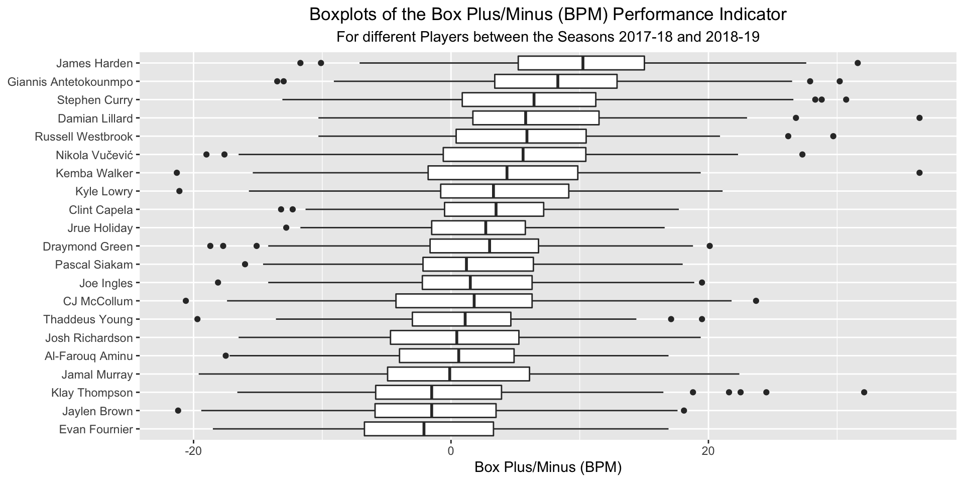
Knowing that the BPM values were normally distributed for the different players, it was sufficient to simply construct boxplots for the performance indicator to get a sense how the individual players performed in general in the two considered seasons and how their performance fluctuated.

4.4 Relationship between the Average 24-Hour Tweet Sentiment and the BPM Performance Indicator

We included a RShiny App to showcase each players correlation between BPM performance and each tweet sentiment. Starting up the app may take some time.

As one can see, the points of the different scatterplots appeared rather scattered. For the different sentiment lexica and players there was neither a strong nor directly visible (linear) relationship between the average tweet sentiment and the BPM performance indicator. Even though some of the linear regression lines suggested a correlation, the correlations themselves were rather weak or even neglectable as indicated by the respective Pearson correlation coefficients r that were relatively small (mostly less than 0.1). Additionally most of the p-values of the associated Pearson correlation coefficients were rather high which suggested that the observed strength of the correlations were not significantly different from 0 (and might have appeared due to random chance).

Nevertheless, there were also some counter examples where the Pearson correlation coefficient appeared rather significant. The player Jaylen Brown for example showed a positive correlation for the Afinn lexicon with a p-value below 0.05. However, since the correlations were rather weak, not significant and somehow contradicting for other sentiment lexica (compare that the correlation was negative for the nrc lexicon), it is debatable if the positive correlation is generalizable for the entire population or even the single player alone.

Due to these reasons we had to conclude that there is no evidence of a significantly strong linear correlation between the average sentiment of tweets, players receive within 24 hours before games and their performance within the games.

There was however another interesting observation the scatterplots revealed, namely the prominent outliers. For almost every player there was at least one game day in which the average tweet sentiment was vastly more positive compared to other days. Additionally there were some players with game days associated with an extremely negative average tweet sentiment in comparison to other days. To investigate these outliers more closely we created two word clouds for each player, one for the smallest average tweet sentiment the player received and one for the highest. We used the tweet sentiments created from the Jockers-Rinker lexicon for this purpose. On extremely positive sentiment values (outliers) the player had birthday. This RShiny App showcases the wordclouds for each player.

The most prominent observation derived from the wordclouds was that the best average sentiments were frequently associated with the words “happy” and “birthday”, which indicated that these players were receiving birthday wishes on that same game day. Besides birthdays it appeared that other players received positive tweet sentiments due to another important day or event in their life. For Stephen Curry the terms “baby”, “congrats”, “boy”, “family”, “hands”, “blue” and “eyes” occurred rather frequently. People were congratulating him for another baby that was on the way.